Getting Started with Methylation-based Inference of Regulatory Activity
John Lawson
2017-09-21
This vignette gives a broad overview of MIRA. For a more realistic example workflow, see the vignette “Applying MIRA to a Biological Question.”
MIRA Overview
MIRA (Methylation-based Inference of Regulatory Activity) is an R package that infers regulatory activity from DNA methylation data. It does this by aggregating DNA methylation data from a set of regions across the genome, producing a single summary profile of DNA methylation for those regions. MIRA then uses this profile to produce a score (the MIRA score) that infers the level of regulatory activity on the basis of the shape of the DNA methylation profile. The region set is provided by the user and should contain regions that correspond to a shared feature, such as binding of a particular transcription factor or DNase hypersensitivity sites. The concept of MIRA relies on the observation that methylation tends to be lower in regions where transcription factors are bound. Since methylation will generally be lower in active regions, the shape of the MIRA signature and the associated score can be used as a metric to compare regulatory activity in different samples and conditions. MIRA thus allows one to predict transcription factor activity data given only DNA methylation data as input. MIRA works with genome-scale, single-nucleotide-resolution methylation data, such as reduced representation bisulfite sequencing (RRBS) or whole genome bisulfite sequencing (WGBS) data. MIRA overcomes sparsity in DNA methylation data by aggregating across many regions. Below are examples of methylation profiles and associated MIRA scores for two (contrived) samples. This vignette will demonstrate how to obtain a methylation profile and MIRA score from the starting inputs of DNA methylation data and a region set.
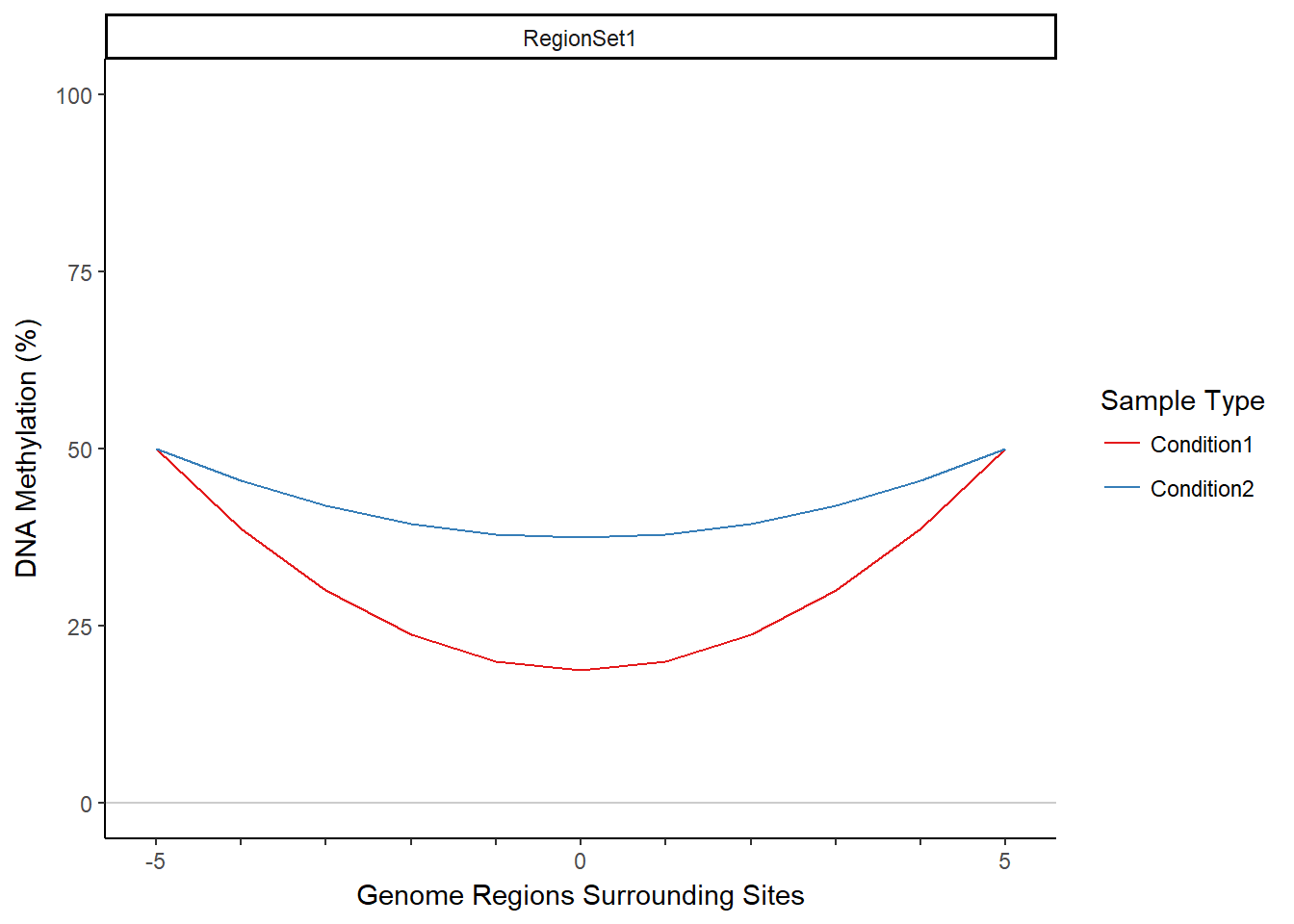
## Warning in summary.lm(wideFit): essentially perfect fit: summary may be
## unreliable

## Warning in summary.lm(wideFit): essentially perfect fit: summary may be
## unreliable
## featureID sampleName score sampleType
## 1: RegionSet1 Sample1 0.9808293 Condition1
## 2: RegionSet1 Sample2 0.2876821 Condition2Required Inputs
You need 2 things to run MIRA:
- Nucleotide-resolution DNA methylation data (in a table with counts methylated and total reads)
- A set of regions
Let’s describe each one in more detail:
DNA Methylation Data
MIRA requires DNA methylation data after methylation calling. For a given genomic coordinate (the location of the C in a CpG), MIRA needs the methylation level (0 to 1) and optionally the total number of reads covering that coordinate which can be used for screening purposes. This data should be represented as a data.table for each sample, which we call a BSDT (Bisulfite data.table). The BSDT will have these columns: chr, start (the coordinate of the C of the CpG) and the methylProp column with methylation level at each cytosine. Alternatively, the methylProp column may be generated from methylCount (number of methylated reads) and coverage (total number of reads covering this site) columns where methylProp = methylCount/coverage and these columns may be included in the data.table addition to the methylProp column. A sampleName (sample identifier) column is optional if there is only one sample but required if you have multiple samples. Since some existing R packages for DNA methylation use different formats, we include a format conversion function that can be used to convert SummarizedExperiment-based objects like you would obtain from the bsseq, methylPipe, and BiSeq packages to the necessary format for MIRA (SummarizedExperimentToDataTable function). A BSseq object is an acceptable input to MIRA and will be converted to the right format internally but for the sake of parallelization it is recommended that BSseq objects be converted to the right format outside the MIRA function so that MIRA can be run on each sample in parallel. Here is an example of a data.table in the right format for input to MIRA:
data("exampleBSDT", package="MIRA")
head(exampleBSDT)
## chr start methylCount coverage sampleName
## 1: chr1 1062326 0 3 Gm06990_1
## 2: chr1 1062330 0 3 Gm06990_1
## 3: chr1 1062339 0 4 Gm06990_1
## 4: chr1 1062448 2 27 Gm06990_1
## 5: chr1 1062478 0 23 Gm06990_1
## 6: chr1 1062480 0 19 Gm06990_1Region Sets
A region set is a GRanges object containing genomic regions that share a biological annotation. For example, it could be ChIP peaks for a transcription factor. Many types of region sets may be used with MIRA, including ChIP regions for transcription factors or histone modifications, promoters for a set of related genes, sites of motif matches, or DNase hypersensitivity sites. Many such region sets may be found in online repositories and we have pulled together some major sources at http://databio.org/regiondb. You may also want to check out the AnnotationHub Bioconductor package which gives access to many region sets in an R-friendly format. For use in MIRA, each region set should be a GRanges object and multiple region sets may be passed to MIRA as a GRangesList with each list element being a region set. Here is an example of a region set, which we will use in this vignette:
data("exampleRegionSet", package="MIRA")
head(exampleRegionSet)
## GRanges object with 6 ranges and 0 metadata columns:
## seqnames ranges strand
## <Rle> <IRanges> <Rle>
## 2763 chr1 [1064067, 1064582] *
## 2433 chr1 [1307973, 1308488] *
## 2948 chr1 [1374984, 1375499] *
## 3845 chr1 [1778779, 1779294] *
## 430 chr1 [1780451, 1780653] *
## 2249 chr1 [2578251, 2578766] *
## -------
## seqinfo: 36 sequences from an unspecified genome; no seqlengthsAnalysis Workflow
The general workflow is as follows:
1. Data inputs: start with single-nucleotide resolution methylation data and one or more sets of genomic regions, as described above. 2. Expand the regions sizes so that MIRA will be able to get a broad methylation profile surrounding your feature of interest. 3. Aggregate methylation data across regions to get a MIRA signature. 4. Calculate MIRA score based on shape of MIRA signature.
The Input
First let’s load the necessary libraries and example data. exampleBSDT is a data.table containing genomic location, methylation hit number, and read number from bisulfite sequencing of a lymphoblastoid cell line. exampleRegionSet is a GRanges object with regions that share a biological annotation, in this case Nrf1 binding in a different lymphoblastoid cell line.
library(MIRA)
library(GenomicRanges) # for the `resize`, `width` functions
data("exampleRegionSet", package="MIRA")
data("exampleBSDT", package="MIRA")
BSDTList = list(exampleBSDT)
Since our input methylation data did not have a column for proportion of methylation at each site (methylProp), we need to add this based on the methylation count and total coverage data.
BSDTList = addMethPropCol(BSDTList)Expand Your Regions
A short but important step. MIRA scores are based on the difference between methylation surrounding the regions versus the methylation at the region itself, so we need to expand our regions to include surrounding bases. Let’s use the resize function from the GenomicRanges package to increase the size of our regions. The average size of our regions is about 500:
mean(width(exampleRegionSet))## [1] 498.788For this vignette, 4000 bp regions should be wide enough to capture the dip:
exampleRegionSet = resize(exampleRegionSet, 4000, fix="center")
mean(width(exampleRegionSet))
## [1] 4000Normally, we want to have each region set (only one in our case) be an item in a list, with corresponding names given to the list:
exampleRegionSet = GRangesList(exampleRegionSet)
names(exampleRegionSet) <- "lymphoblastoid_NRF1"
Aggregation of Methylation across Regions
Next we aggregate the methylation across regions to get a summary methylation profile with the aggregateMethyl function. MIRA divides each region into bins, finds methylation that is contained in each bin in each region, and aggregates matching bins over all the regions (all 1st bins together, 2nd bins together, etc.). A couple important parameters: The binNum argument determines how many approximately equally sized bins each region is split into. This could affect the resolution or noisiness of the MIRA signature because using more bins will result in smaller bin sizes (potentially increasing resolution) but also less reads per bin (potentially increasing noise). The minReads argument in aggregateMethyl is used to screen out region sets that have any bins with fewer than a minimum number of reads. Here we use the default (500). Let’s aggregate the methylation and then view the MIRA signature.
bigBin = lapply(X=BSDTList, FUN=aggregateMethyl, GRList=exampleRegionSet,
                binNum=11)
bigBinDT = bigBin[[1]]
plotMIRAProfiles(binnedRegDT=bigBinDT)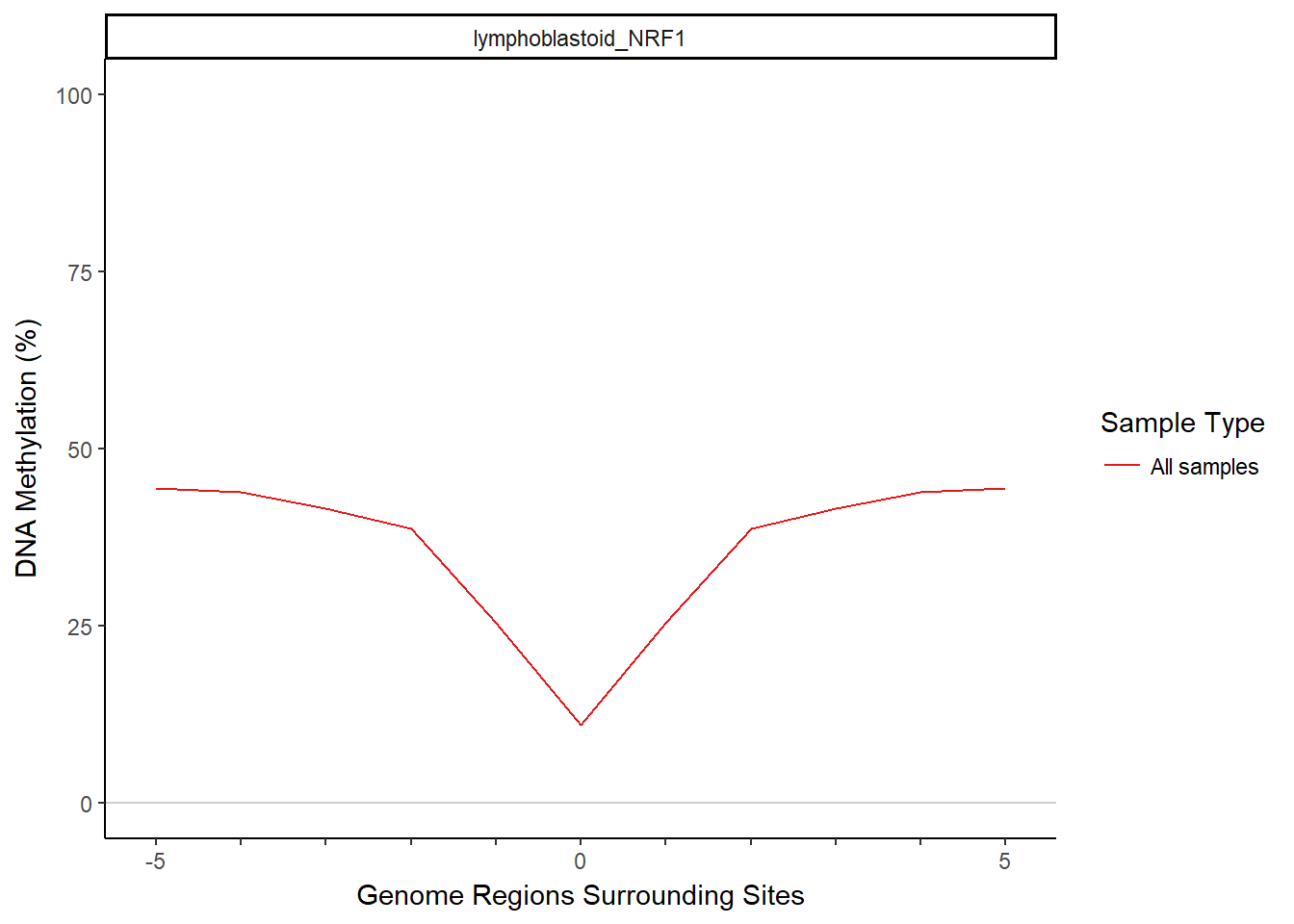
Calculating the MIRA Score
To calculate MIRA scores based on the MIRA signatures, we will apply the scoring function, scoreDip, to the data.table that contains the methylation aggregated in bins. scoreDip calculates a score for each group of bins corresponding to a sample and region set, based on the degree of the dip in the signature. With MIRA’s default scoring method (logratio), scoreDip will take the log of the ratio of the outside edges of the dip to the center of the dip. Higher MIRA scores are associated with deeper dips. A flat MIRA signature would have a score of 0.
sampleScores = scoreDip(bigBinDT,
                        regionSetIDColName = "featureID",
                        sampleIDColName = "sampleName")
head(sampleScores)
## featureID sampleName score
## 1: lymphoblastoid_NRF1 Gm06990_1 1.393596A Note on Annotation
For real uses of MIRA, samples and region sets should be annotated. The data.table for each sample should include a sampleName column while region sets should be given to MIRA in a named list/GRangesList. An annotation file that matches sample name with sample type (sampleType column) can be used to add sample type information to the data.table after aggregating methylation. A sampleType column is not required for the main functions but is used for the plotting functions. See “Applying MIRA to a Biological Question” vignette for a workflow including annotation.
Interpreting the Results
Regulatory information can be inferred from the MIRA scores and signatures but interpretation depends on the type of region set and samples used. The basic assumption is that deeper dips and higher MIRA scores would be associated with generally higher activity at the regions that were tested, which might also inform you about the activity of the regulatory feature that defines the region set (eg the activity of a transcription factor if using ChIP-seq regions). However, MIRA does not directly tell you the activity of the regulatory feature and, in some cases, higher MIRA scores will not be associated with higher activity of the regulatory feature. For example, samples with higher MIRA scores for a transcription factor binding region set could have more activity of that transcription factor but there could be other causes like increased activity of a different transcription factor that binds to many of the same regions or the fact that the samples with higher scores generally had more similar chromatin states to the samples from which the region set was derived than samples with lower scores did (eg when using MIRA on samples from multiple tissue/cell types and the region set was derived from the same tissue/cell type as some but not all of the samples). The general interpretation rule though is a higher MIRA score means more activity (although what kind of activity depends on the context). For more on interpreting the results, see the “Applying MIRA to a Biological Question” vignette.