Applying MIRA to a Biological Question
John Lawson
2017-09-21
In this vignette, we show a more realistic MIRA workflow, including adding annotation and using multiple samples and region sets. Only the second half of this vignette is evaluated because of the large files involved.
Biological Question
Ewing sarcoma is a pediatric cancer defined by the fusion oncoprotein EWS-FLI1, a transcription factor. We have DNA methylation data for Ewing sarcoma and muscle-related samples and we want to use this data to see if Ewing samples can be distinguished from muscle-related samples. We’re also interested in exploring the regulatory activity of different genomic regions. MIRA can aggregate methylation from regions of interest across the genome which share some biological annotation (like transcription factor ChIP regions or DNase hypersensitivy sites (DHSs) for instance) in order to get a summary methylation profile for those regions. The MIRA package relies on the assumption that active genomic regions will tend to have lower DNA methylation levels due to binding of transcription factors and a more open chromatin state so the shape of the methylation profile contains information about the activity of those regions. You can infer differences between samples in the regulatory activity of those regions by comparing the profiles and associated scores (which are calculated based on the shape of the profiles). We will compare the Ewing samples to the muscle samples using MIRA with two region sets: first, Ewing-specific DHSs, and second, muscle-specific DHSs.
Input:
This vignette requires large input files, which can be dowloaded here: MIRA_Ewing_Vignette_Files.tgz. This archive contains:
- Single-nucleotide resolution DNA methylation data (RRBS data) for 12 Ewing sarcoma samples and 12 myotube (muscle) samples recently analyzed in the paper DNA methylation heterogeneity defines a disease spectrum in Ewing sarcoma.
- Two sets of regions – one with Ewing-specific DHSs and a one with muscle-specific DHSs, obtained from the Regulatory Elements Database. All data is on the hg38 reference genome.
Package workflow
Preparation: Start with appropriately formatted single-nucleotide resolution methylation data, region sets – each with genomic regions corresponding to some biological annotation, and a sample annotation file that has sample name (sampleName column) and sample type (sampleType column). See ?SummarizedExperimentToDataTable for options for converting formats from some other DNA methylation packages to our format.
1. Do a quick run-through of the MIRA workflow with each region set with a few samples from each condition/sample type to make sure the region sizes are reasonable (discussed later).
1.1. Aggregate methylation data across regions to get a MIRA signature for each region set, sample combination.
1.2. Calculate MIRA score for each region set, sample combination based on the shape of the MIRA signature.
2. Based on preliminary results, pick a region size for each region set depending on what the MIRA signatures look like.
3. Run the full MIRA analysis with chosen region sizes.
3.1. Aggregate methylation data across regions to get a MIRA signature for each region set, sample combination.
3.2. Calculate MIRA score for each region set, sample combination based on the shape of the MIRA signature.
Initial Run-through
First, let’s load the libraries and read in the data files. A sample annotation file was included with the package:
library(MIRA)
library(data.table) # for the functions: fread, setkey, merge
library(GenomicRanges) # for the functions: GRanges, resize
library(ggplot2) # for the function: ylab
exampleAnnoDT2 = fread(system.file("extdata", "exampleAnnoDT2.txt",
                                   package="MIRA"))
Next, construct file names for the DNA methylation samples and the region sets (downloaded through the link in the Input section).
# 12 Ewing samples: T1-T12
pathToData="/path/to/MIRA_Ewing_Vignette_Files/"
ewingFiles = paste0(pathToData, "EWS_T", 1:12, ".bed")
# 12 muscle related samples, 3 of each type
muscleFiles = c("Hsmm_", "Hsmmt_", "Hsmmfshd_","Hsmmtubefshd_")
muscleFiles = paste0(pathToData, muscleFiles, rep(1:3, each=4), ".bed")
RRBSFiles = c(ewingFiles, muscleFiles)
regionSetFiles = paste0(pathToData, c("sknmc_specific.bed", "muscle_specific.bed"))
Let’s read the files into R:
BSDTList = lapply(X=RRBSFiles, FUN=BSreadBiSeq)
regionSets = lapply(X=regionSetFiles, FUN=fread)
We need to do a bit of preprocessing before we plug the data into MIRA. The BSreadBiSeq function reads DNA methylation calls from the software Biseqmethcalling, reading the methylation calls into data.table objects. We read in the region sets with fread so they will also be data.table objects. Let’s convert the region sets from data.table objects to GRanges objects, including chromosome, start, and end info. In most cases, strand information is not needed by MIRA and should be omitted.
regionSets = lapply(X=regionSets,
                    FUN=function(x) setNames(x, c("chr", "start", "end")))
regionSets = lapply(X=regionSets, FUN=
                        function(x) GRanges(seqnames=x$chr,
                                              ranges=IRanges(x$start, x$end)))
We also need to pick initial region sizes. To get the methylation profile around our sites of interest, we are resizing the regions to 5000 bp. This is a wide initial guess compared to the average region sizes for the region sets (around 151 bp for both region sets), but we will adjust this later on.
regionSets[[1]] = resize(regionSets[[1]], 5000, fix="center")
regionSets[[2]] = resize(regionSets[[2]], 5000, fix="center")
names(regionSets) = c("Ewing_Specific", "Muscle_Specific")
Now we are ready to run MIRA on a subset of the samples – three Ewing and three muscle samples. First, we aggregate the methylation data into bins with aggregateMethyl. MIRA divides each region into bins and finds methylation that is contained in each bin in each region. Then matching bins are aggregated over all regions (all bin1’s together, all bin2’s together, etc.). The bin number (binNum) will affect the resolution or noisiness of the data – a higher bin number will allow more resolution since each bin will correspond to a smaller genomic region but with the trade-off of possibly increasing noise due to less methylation data in each bin. An odd bin number is recommended for the sake of symmetry and MIRA scoring.
subBSDTList = BSDTList[c(1, 5, 9, 13, 17, 21)]
bigBin = lapply(X=subBSDTList, FUN=aggregateMethyl, GRList=regionSets,
                binNum=21, minReads=0)
bigBinDT1 = rbindlist(bigBin)
If you are running the actual samples on your own device, you can skip the following step. Otherwise, let’s load the binned methylation data (bigBinDT1) that would have been obtained by the previous step.
# from data included with MIRA package
data(bigBinDT1)
Next we add on annotation data: the experimental condition or sample type for each sample. This is needed in order to group samples by sample type, which we will do when plotting the methylation profiles and MIRA scores. We will use functions from the data.table package to do this, merging based on the sampleName column.
setkey(exampleAnnoDT2, sampleName)
setkey(bigBinDT1, sampleName)
bigBinDT1 = merge(bigBinDT1, exampleAnnoDT2, all.x=TRUE)
Let’s look at the MIRA signatures to see if we should change our region sizes.
plotMIRAProfiles(binnedRegDT=bigBinDT1)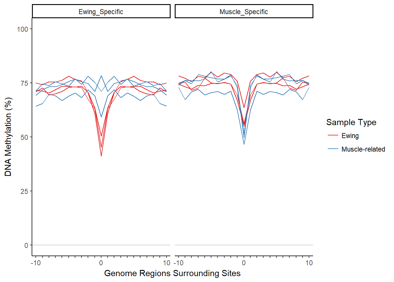
Choosing Appropriate Region Sizes
While the methylation profiles look pretty good, the dips are a bit too narrow for the muscle-related samples when looking at the muscle-specific region set. The scoring function in MIRA could run into problems if the dips are too narrow since it expects the dips to be at least 5 bins wide from outside edge to outside edge (that number includes the outside edges). Let’s use smaller region sizes for both region sets: 4000 bp for the Ewing DHS regions and 1750 bp for the muscle DHS regions (the choice is somewhat arbitrary). The size of the regions should not be decreased too much; if the regions are too small, there might be more noise since there would be less methylation data for each bin. Also, the regions must be wide enough to capture the outer edges of the dip since the outer edges are used for the MIRA score.
To implement our new region sizes:
regionSets[[1]] = resize(regionSets[[1]], 4000, fix="center") # Ewing
regionSets[[2]] = resize(regionSets[[2]], 1750, fix="center") # muscle
Full MIRA Analysis
Now we can run MIRA with all our samples. Let’s aggregate methylation data again with aggregateMethyl.
bigBin = lapply(X=BSDTList, FUN=aggregateMethyl, GRList=regionSets,
                binNum=21, minReads=0)
bigBinDT2 = rbindlist(bigBin)
If you are running the actual samples on your own device, you can skip the following step. Otherwise, let’s load the binned methylation data (bigBinDT2) that would have been obtained by the previous step.
# from data included with MIRA package
data(bigBinDT2)
We add annotation data using the same process as before:
# data.table functions are used to add info from annotation object to bigBinDT2
setkey(exampleAnnoDT2, sampleName)
setkey(bigBinDT2, sampleName)
bigBinDT2 = merge(bigBinDT2, exampleAnnoDT2, all.x=TRUE)
Let’s look at the MIRA signatures:
plotMIRAProfiles(binnedRegDT=bigBinDT2)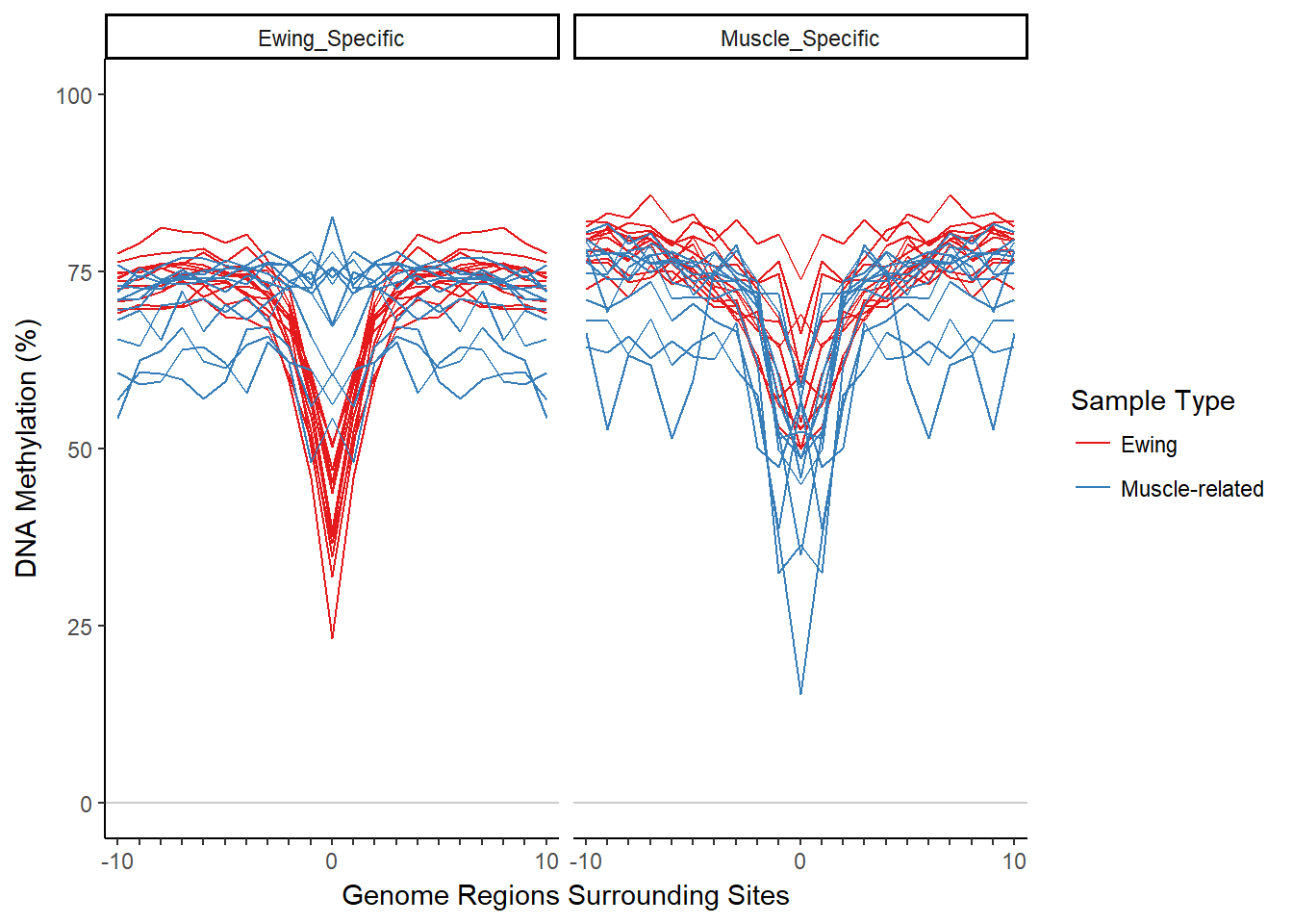
Next we normalize the binned methylation data (the MIRA signature). Normalizing by subtracting the minimum methylation bin value from each sample/region set combination generally brings the center MIRA signatures to a similar methylation value, making the MIRA score more about the shape of the signature and less about the average methylation. We do this with data.table syntax.
bigBinDT2[, methylProp := methylProp - min(methylProp) + .05, by=.(featureID, sampleName)]normPlot = plotMIRAProfiles(binnedRegDT=bigBinDT2)
normPlot + ylab("Normalized DNA Methylation (%)")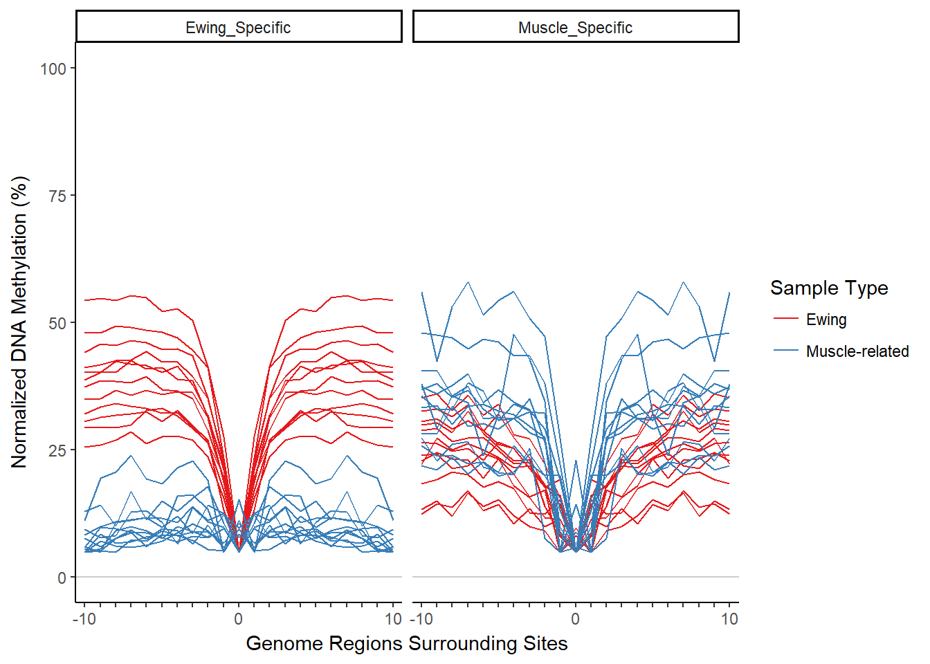
Now we can calculate MIRA scores for all samples with the scoreDip function.
sampleScores = scoreDip(bigBinDT2,
                        shoulderShift="auto",
                        regionSetIDColName = "featureID",
                        sampleIDColName = "sampleName")
head(sampleScores)
## featureID sampleName score
## 1: Ewing_Specific EWS_T1 2.180698
## 2: Ewing_Specific EWS_T10 2.114649
## 3: Ewing_Specific EWS_T11 2.064900
## 4: Ewing_Specific EWS_T12 2.290313
## 5: Ewing_Specific EWS_T2 1.987881
## 6: Ewing_Specific EWS_T3 2.230074Finally, let’s add the annotation data back on and take a look at the scores!
setkey(exampleAnnoDT2, sampleName)
setkey(sampleScores, sampleName)
sampleScores = merge(sampleScores, exampleAnnoDT2, all.x=TRUE)
plotMIRAScores(sampleScores)
Interpreting the Results
As expected, we found that the Ewing sarcoma samples had higher MIRA scores for the Ewing-specific DHSs, which implies more activity in Ewing-specific regions. The muscle-specific DHSs require more interpretation. The muscle samples on average had higher MIRA scores but there was not complete separation between the groups. This suggests that the Ewing samples still have some activity in muscle-specific regions.
General Interpretation Tips and Caveats
In general, interpretation will depend on the samples and region sets being used. While we have found MIRA useful for inferring regulatory activity of transcription factors, we must also remember that the MIRA score is only an indirect inference of activity of the TF. The methylation profile could be affected by other TFs aside from the TF of interest. Thus, it is possible that a sample could have a higher MIRA score for TF-binding regions than another sample yet still have less activity for that TF (but perhaps more activity for other regulatory elements that happen to also be in the same regions). With TF-binding region sets, what we are really measuring is simply that the regions where the TF binds have altered activity in one sample relative to another sample. The main thing to remember is that MIRA infers the general regulatory activity of the regions you give it and the biological interpretation depends on the samples and type of regions (biological annotation as well as the source tissue/cell type) you use.
Other Tips for Using MIRA
When it comes to MIRA, lapply is your friend (although this is generally true anyway). This allows for distributed computing with mclapply (parallel package) or bplapply (BiocParallel package) if desired.